Supplementary material
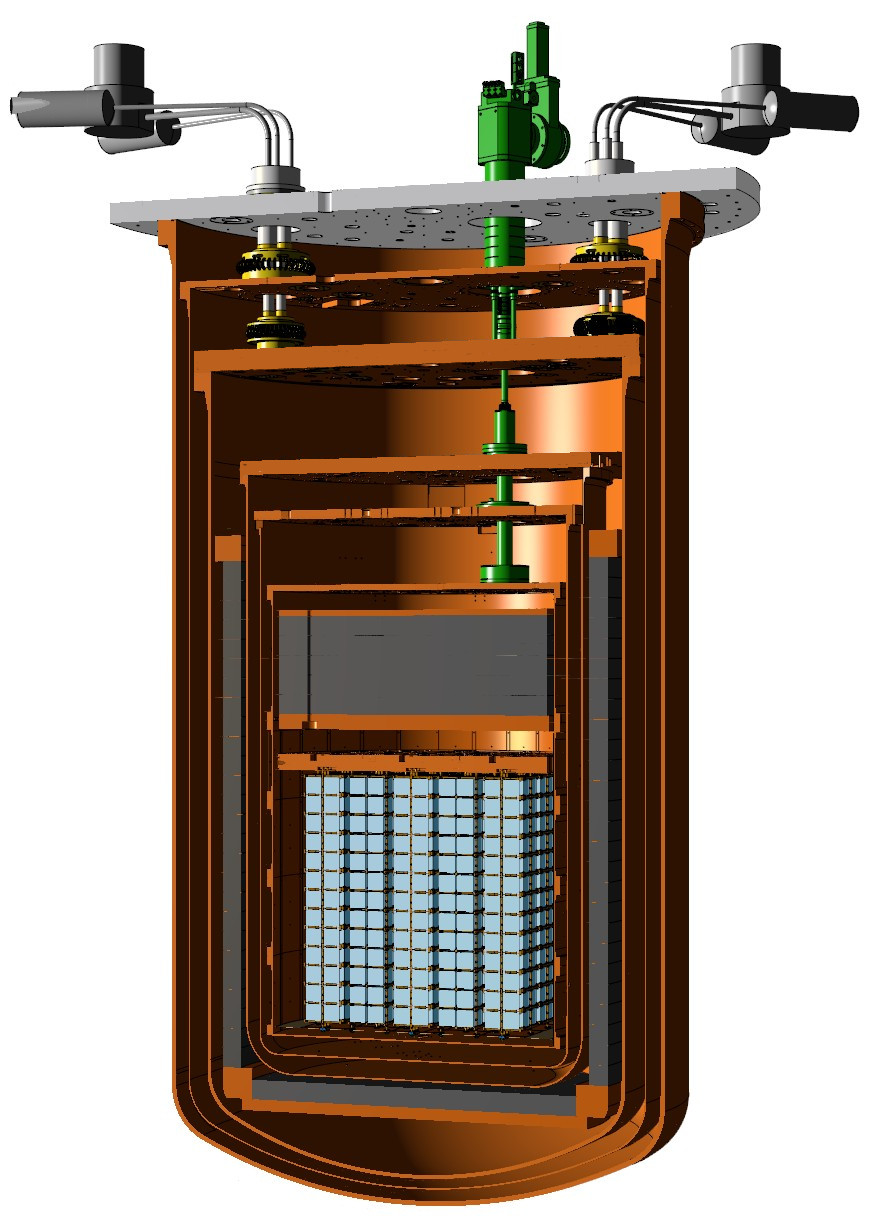
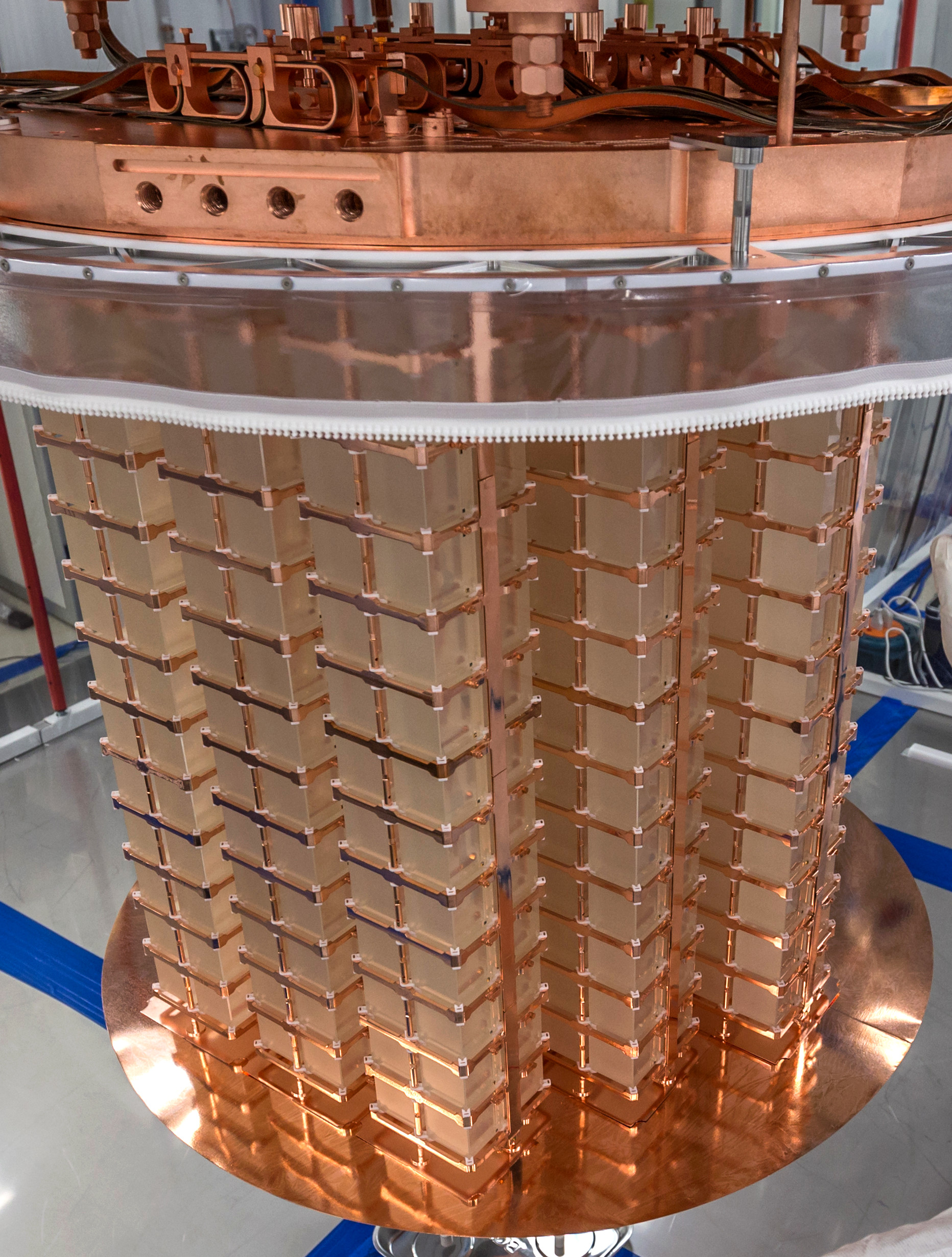
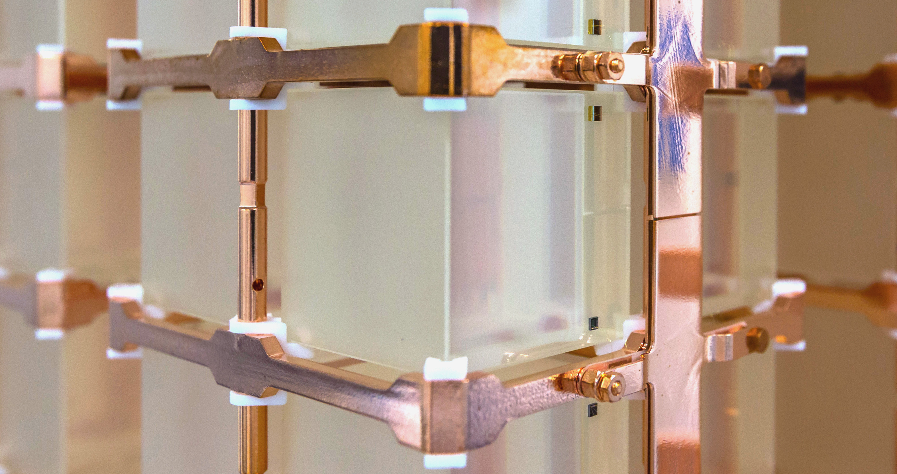
Figure 1

Figure 1
   
The CUORE detector. Left: Rendering of the 6-stage cryostat, with the pulse tubes and dilution unit, the internal low-radioactivity modern and Roman lead shields, and the array of 988 TeO2 crystals (light blue). Top right: The detector after installation. The plastic ring was used during assembly for radon protection. Bottom right: One of the calorimeters instrumented with an NTD Ge thermistor which measures the temperature increase induced by absorbed radiation. The Si heater is used to inject pulses for thermal gain stabilization. The PTFE supports and the gold wires instrumenting the NTD and the heater provide the thermal link between the crystal and the heat bath, i.e. the Cu frames.
PDF
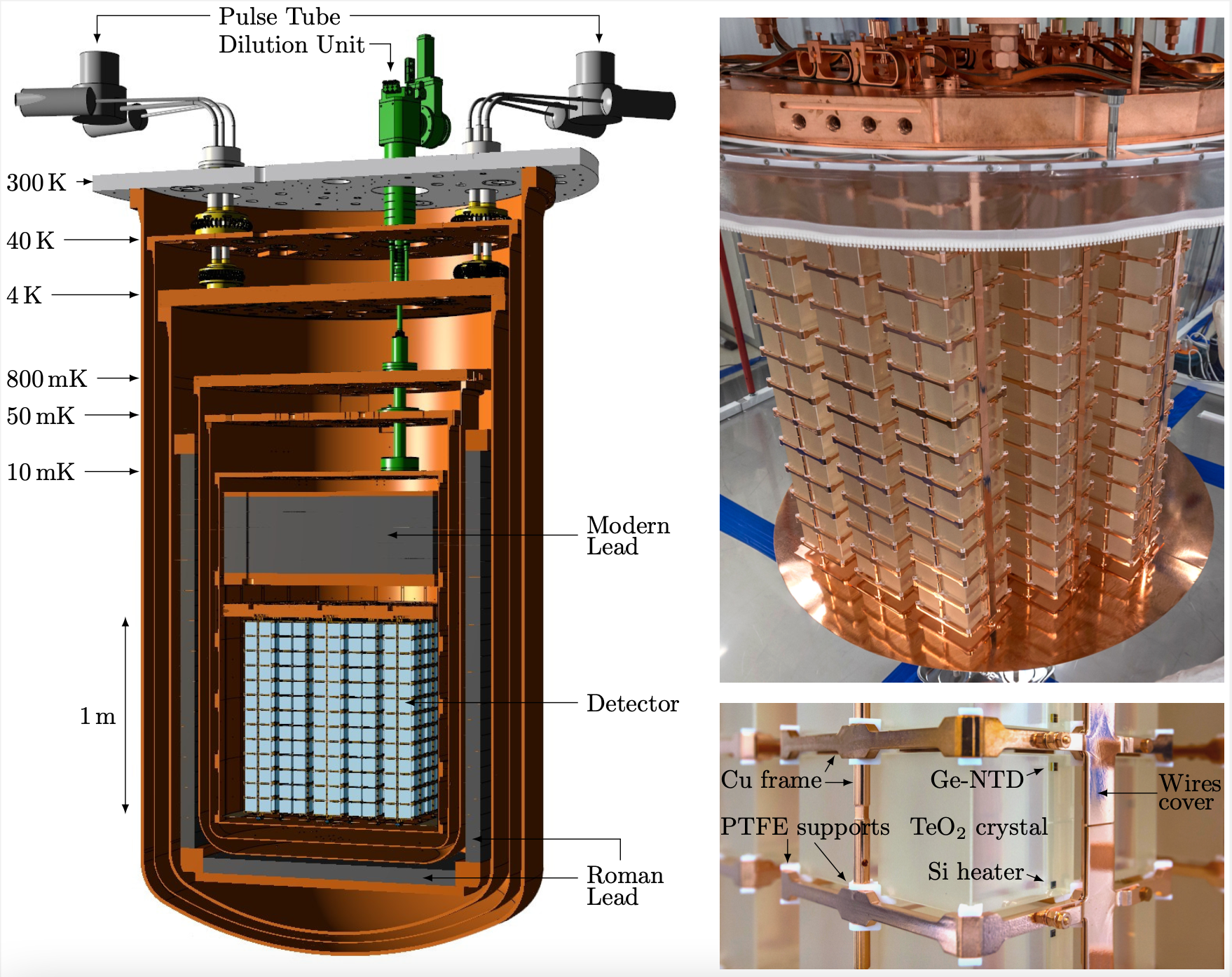
JPEG (cryostat rendering) JPEG (detector) JPEG (CUORE crystal)

Figure 2

Cryostat performance
   
Cryogenic performance. Top: The exposure accumulated by CUORE (left, teal), along with the exposure used for this analysis (left, orange). Middle: Examples of common temperature instabilities induced by external causes, e.g. blackouts and earthquakes, or human intervention, such as regular maintenance or the insertion of calibration sources.
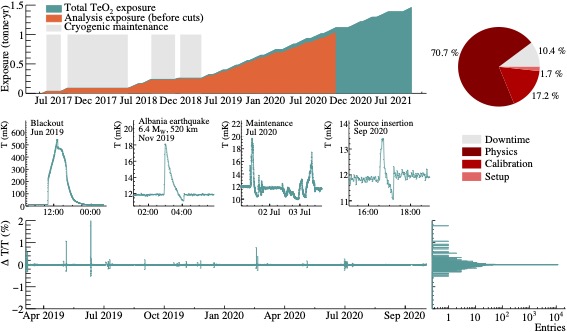
Bottom: The temperature stability of CUORE over ~1 yr of continuous operation.
JPEG PDF
CSV (middle - blackout) CSV (middle - earthquake) CSV (middle - maintenance) CSV (middle - source insertion)
CSV (top) CSV (bottom)

Figure 3

PT phase optimization
   
PT phase optimization. Top: frequency spectrum of the noise for a random combination of the PT phases (orange) and after the active phase tuning (teal). The frequency spectrum of physical signals is also reported for reference. Bottom: integral of the power spectrum at the PT frequency (1.4 Hz) and its harmonics before and after active noise cancellation.
PDF
CSV (top) CSV (bottom)

Figure 4

Physics spectrum for 1038 kg yr exposure
   
Physics spectrum for 1038.4 kg · yr of TeO2 exposure in counts/(keV kg yr). We separately show the effects of the base cuts, the anti-coincidence (AC) cut, and the pulse shape discrimination (PSD). The most prominent background peaks in the spectrum are highlighted. Top right inset: the ROI after all selection cuts, with the best-fit curve (solid red), the best-fit curve with the 0νββ rate fixed to the 90% CI limit (blue), and background-only fit (black) superimposed.
PDF
CSV CSV (inset)

Extended Data Figure 1

Extended Data Figure 1
   
Working principle of the cryogenic calorimeter. Left: simplified calorimeter thermal model. The detector is modeled as a single object with heat capacity C coupled to the heat bath (with constant temperature T0) through the thermal conductance G. The NTD thermistor for signal readout is glued to the absorber. Right: Example of a CUORE pulse from the 2615 keV calibration line: T0 corresponds to the baseline height, the pulse amplitude is proportional to the deposited energy, and the decay time depends on the C/G ratio.
PDF
CSV (CUORE pulse) PDF (CUORE pulse)

Extended Data Figure 2

Extended Data Figure 2
   
Roman lead. Top left: the lead bricks recovery from the Sardinian sea. Bottom left: the ingot inscriptions were cut and preserved, while the ingot bodies were used for the CUORE internal lead shield. Right: Lateral view of the internal lead shield.
PDF
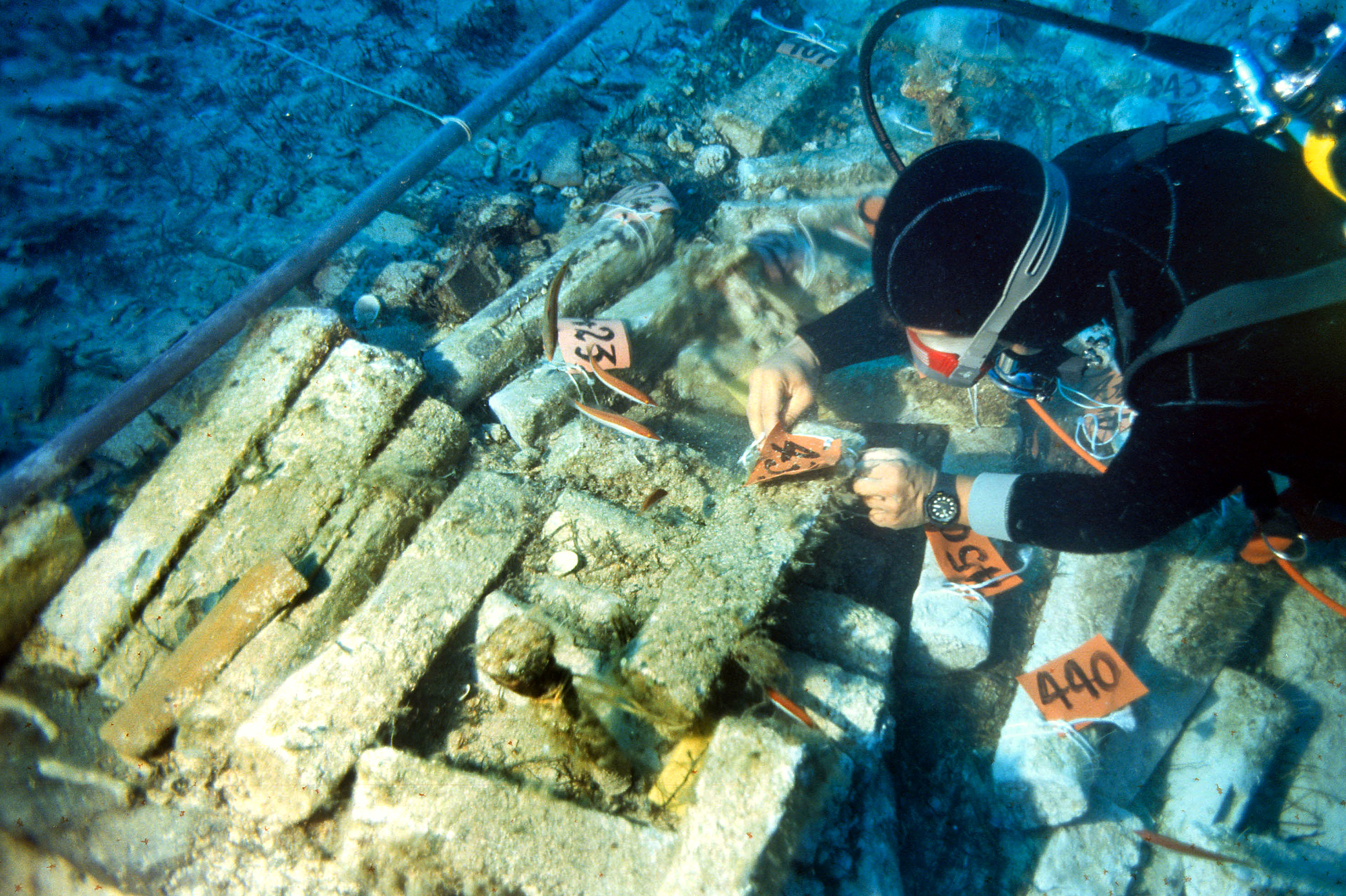
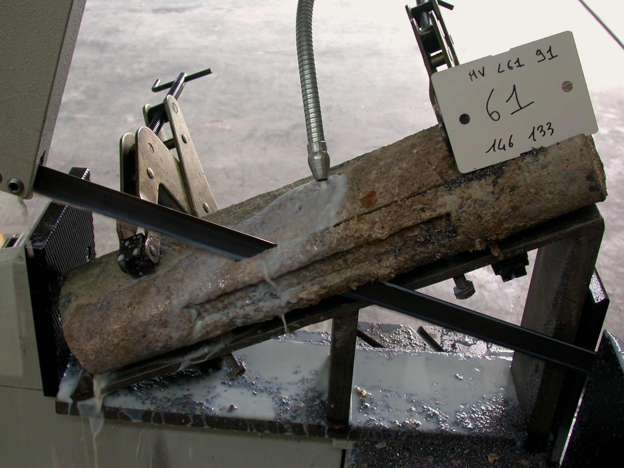
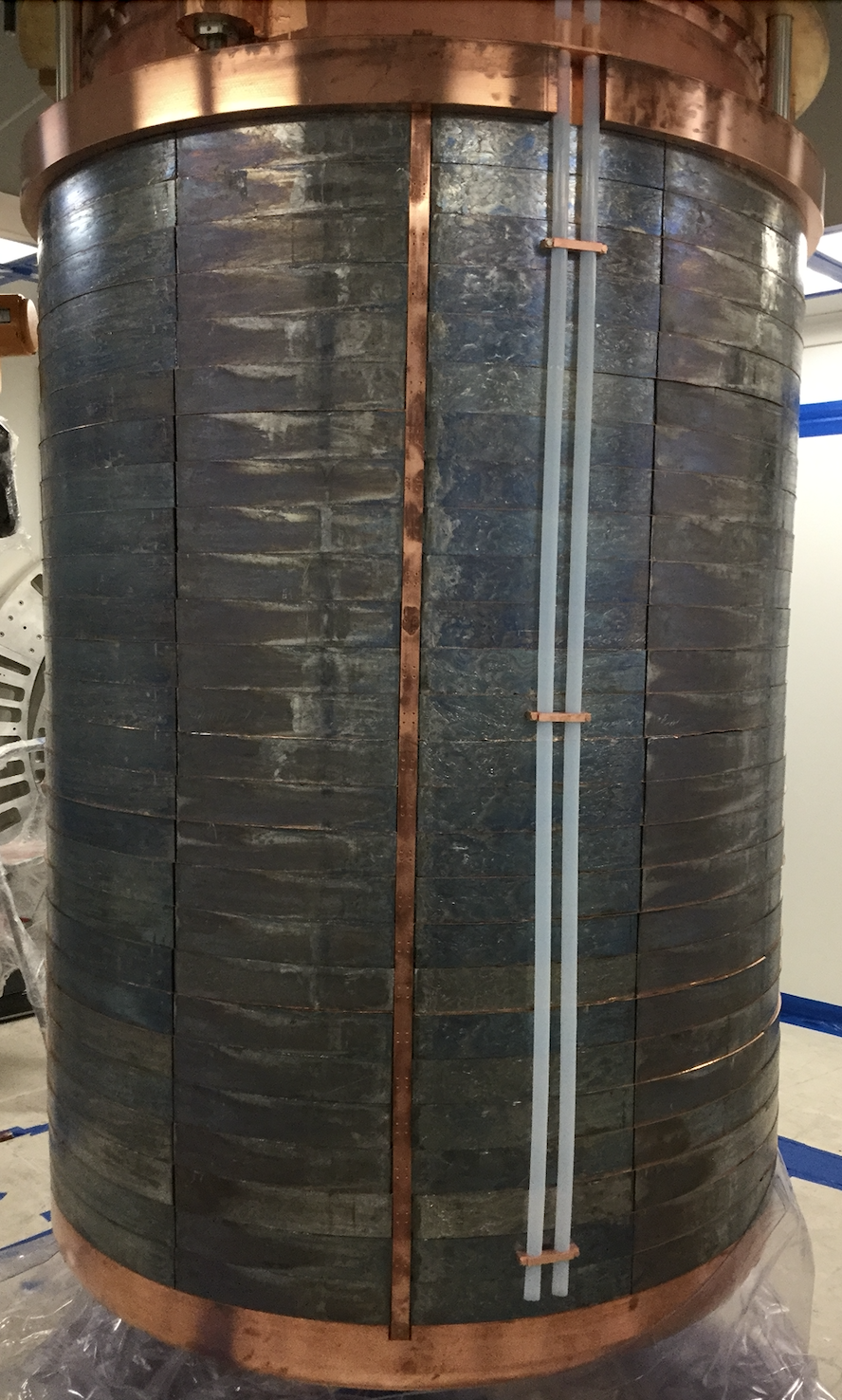
JPEG (Roman lead under the sea) JPEG (Roman lead cutting) PNG (Roman lead shield)

Extended Data Figure 3

Pulse Shape Discrimination
   
Pulse Shape Discrimination. Effect of the PSD cut on calibration data around the 2615 keV line (left) and on physics data near Qββ (right). In calibration data, the AC is not applied in order to maximize the statistics on the γ peaks, and the PSD mostly removes pileup events (events with more than one energy deposit in the time window). In physics data, the PSD mostly eliminates random noise events, which can correspond to either physical events with excessive noise or to noise-induced events with non-physical pulse shapes.
Such events appear randomly across the energy spectrum, so the cut mostly acts on the continuum.
PDF
CSV (calibration) CSV (physics)

Extended Data Figure 4

Trigger and High Level Analysis
   
Optimum trigger and statistical analysis. Top left: Distribution of energy thresholds at 90% trigger efficiency for the OT algorithm in a single dataset. The 40 keV analysis threshold is indicated by the vertical line. Top right: 90% C.I. exclusion limits on T1/2 from an ensemble of 104 toy experiments generated with the background-only model, with background rates obtained from the background-only fit to the data. The median exclusion sensitivity is indicated by the orange line. Bottom left: Posterior probability distribution for Γ obtained from the Bayesian fit, with the 90% C.I. highlighted. Bottom right: ΔΧ2 values obtained from the profile likelihood of Γ, with ΔΧ2 = 0 being the most-favored value.
The frequentist limit at 90% confidence level (C.L.) is indicated.
PDF
CSV (trigger thresholds) CSV (exclusion sensitivity)
CSV (rate posterior) CSV (profile likelihood)

Extended Data Figure 5

Principal Component Analysis
   
PCA performance. Left: example of a normalization fit of the PCA reconstruction error vs energy for a single calorimeter and dataset. The distribution contains only events that passed the other base cuts. The second order polynomial fit is shown in orange. Right: two example pulses from this calorimeter. The actual pulse is drawn in teal, and the corresponding reconstruction obtained by the PCA is drawn in orange. The top pulse deviates from the expected shape of a good pulse and is rejected, while the bottom one conforms to the expected response and is accepted.
PDF CSV